
Your radar module meets every number on its datasheet. Then it goes into the enclosure, and it starts missing a person standing three metres away.
Nothing in the silicon changed. What changed is everything around it. The laminate the feed line runs on, the copper roughness under the solder mask, the plastic in front of the antenna, the steel bracket bolted beside it. Millimetre wave radar performance belongs to the assembled product, and a module datasheet is measured on a test fixture, not inside your housing.
So the useful way to learn this technology runs in order. Understand what the radio is doing, see where the band choices come from, then follow the signal down into the stack-up and the mechanical design. Get that sequence right and the board decisions stop feeling arbitrary.
Table of Contents
- Millimetre Wave Radar Frequency Bands at a Glance
- How Millimetre Wave Radar Works, Step by Step
- Where Millimetre Wave Radar Is Used Today
- Limits of Penetration, Clutter and Blind Zones
- Choosing PCB Materials for Millimetre Wave Boards
- PCB Layout Checklist for Impedance and Antennas
- Validate the Stack-Up Before You Build Prototypes
<a id="millimetre-wave-radar-frequency-bands-at-a-glance"></a>
Millimetre Wave Radar Frequency Bands at a Glance
Millimetre wave radar transmits and listens in the 30 to 300 GHz range, where free-space wavelengths run from 10 mm down to 1 mm. That short wavelength is the reason the technology fits inside a product at all. An antenna is roughly half a wavelength across, so at 77 GHz, where the wavelength works out to about 3.9 mm, a patch antenna is a few millimetres of copper.
Compare that with a 433 MHz sub-GHz radio, where the antenna is measured in centimetres and usually ships as a wire or a coil. The trade is simple. Higher frequency buys small antennas, wide bandwidth and fine resolution, and it charges you in propagation loss, material loss and tolerance sensitivity. Every band below sits somewhere different on that trade.
| Band | Frequency range | Typical use | Main trade-off | |---|---|---|---| | 24 GHz ISM | 24.00 to 24.25 GHz | Presence and motion sensing, low-cost indoor sensors | Narrow bandwidth limits fine resolution | | 60 GHz | About 57 to 64 GHz, unlicensed in many regions | Gesture, occupancy and vital-sign sensing | Oxygen absorption limits range | | 77 GHz long range | 76 to 77 GHz | Adaptive cruise control and long-range automotive radar | Only 1 GHz of bandwidth in the original allocation | | 76 to 81 GHz automotive | 76 to 81 GHz, 5 GHz contiguous | Short-range automotive functions such as blind-spot detection and parking | Needs tight PCB and antenna control | | 94 GHz W-band | Around 75 to 110 GHz, with 94 GHz the common centre | High-resolution imaging and security screening | Higher atmospheric loss and costlier hardware |
The 24 GHz row explains why cheap motion sensors exist: a few hundred megahertz of bandwidth is enough to answer "is something moving in this room" and not much else. The 60 GHz row is the one that surprises people. Oxygen molecules absorb energy near 60 GHz, which shortens usable range but also makes the band convenient for short-range vital-sign work, where you want the signal to die off before it reaches the neighbours.
Choose from the requirement, not the catalogue. Start with the range you must cover and the resolution you must achieve, then work backwards to the antenna and the laminate.
Practical rule: if two targets sitting close together must be told apart, bandwidth decides it. Antenna gain and processing cleverness won't rescue a narrow sweep.
<a id="how-millimetre-wave-radar-works-step-by-step"></a>
How Millimetre Wave Radar Works, Step by Step
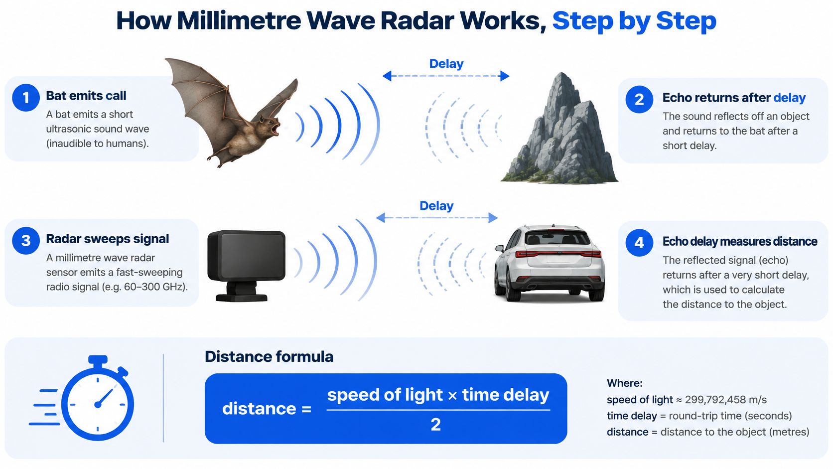
A bat hunts by shouting and listening. The call goes out, the echo comes back, and the delay tells the bat how far away the wall is. A millimetre wave radar does the same thing with a radio signal that sweeps quickly across its band.
<a id="from-chirp-to-detected-target"></a>
From chirp to detected target
The radar is a frequency-modulated continuous wave system, usually shortened to FMCW. Six stages carry a chirp from the transmitter to a decision.
- The transmitter sweeps a chirp. The carrier starts near the bottom of the band and rises steadily, for example a 4 GHz sweep inside 76 to 81 GHz. That sweep is the ruler everything else is measured against.
- The echo comes back late. The signal travels out, reflects off an object, and returns. The round trip takes longer for distant objects, and the delay scales directly with distance.
- The receiver mixes echo against chirp. Multiplying the returned signal by a copy of the transmitted one produces a beat tone. Two nearly identical frequencies mixed together give a slow difference tone, and that tone climbs as the target gets further away.
- Motion leaves a second signature. A hand moving toward the sensor, or a chest wall rising, shifts the return in frequency. Doppler gives radial velocity inside the same frame, with no tracking across frames.
- An FFT builds the range-Doppler map. Range sits on one axis, velocity on the other, and each cell holds received power. Breathing and heartbeats appear as tiny displacements that move the phase of a single cell.
- Detection and tracking decide what's real. A threshold picks peaks, clustering groups them, and a tracker asks whether a peak persists over time. Clutter that flickers and dies gets dropped here.
<a id="what-bandwidth-buys-you-in-centimetres"></a>
What bandwidth buys you in centimetres
Range resolution comes from the sweep, not from the antenna. The relationship is short enough to keep on a sticky note.
Range resolution = c / (2 × B), where c is the speed of light and B is the swept bandwidth. A 4 GHz sweep gives about 3.75 cm, so two objects closer than that blur into one peak.
Widen the sweep and the blur shrinks. That's the whole design argument behind the modern automotive band, where a contiguous block at the top of the spectrum allows sweeps that a 1 GHz allocation could never support.
Angle is a separate problem. Bearing comes from the antenna array and the number of receive channels, not from bandwidth, so a wide sweep with a tiny array still gives you coarse direction.
<a id="what-a-healthy-sensor-looks-like"></a>
What a healthy sensor looks like
Point a working radar at a stationary target at a known distance. You want one clean, stable peak sitting in the correct range bin, a low noise floor either side of it, and a consistent reading over hundreds of frames. If the peak wanders, or lands in the wrong bin, suspect the RF path and the calibration before you rewrite the detection code.
<a id="where-millimetre-wave-radar-is-used-today"></a>
Where Millimetre Wave Radar Is Used Today
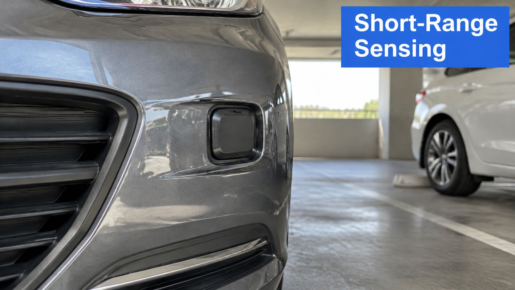
Automotive work drove the technology, and the regulatory timeline explains why the hardware looks the way it does. In 1995, the U.S. Federal Communications Commission authorised vehicle-mounted radar in the 76 to 77 GHz band on an unlicensed basis, according to a Davis Wright Tremaine analysis of the FCC's 76 to 81 GHz decision. Those early systems carried long-range functions such as adaptive cruise control.
Short-range sensing only became practical later. On 13 July 2017, the FCC authorised vehicular radar across the entire 76 to 81 GHz band under an interference-protected framework, with the rules taking effect on 20 October 2017. The wider allocation allowed wideband, high-precision short-range radar while leaving room for long-range adaptive cruise control, and blind-spot monitoring and parking assistance followed.
<a id="one-field-at-a-time-and-why-radar-won"></a>
One field at a time, and why radar won
Industrial plants use radar for tank level measurement and machine safety zones. Steam, dust and washdown kill optical sensors, while a radar keeps reading through the mess. That's the deciding factor, not resolution.
Smart buildings count occupancy and adjust lighting or HVAC without a camera in a meeting room. The selling point is that no identifiable image ever exists, so privacy review gets shorter.
In elder care, a sensor detects falls or changes in breathing rate through clothing and blankets. A camera in a bedroom would be a hard sell to a resident, and a wearable gets taken off. Radar sits in the useful middle.
Perimeter security runs radar in darkness, rain and fog, where a camera needs infrared illumination that gives away its position. Consumer devices use the same physics for gesture control, laptop presence detection and appliances that wake when someone walks in.
<a id="the-matching-rule"></a>
The matching rule
Watch the pattern. Every one of those applications was decided by two numbers, the range it must cover and the resolution it must resolve, and the band follows from that pair.
<iframe width="100%" style="aspect-ratio: 16 / 9;" src="https://www.youtube.com/embed/XJ6JhB8wOPU" frameborder="0" allow="autoplay; encrypted-media" allowfullscreen></iframe>Once the band is fixed, the antenna geometry and the board design follow. A 60 GHz occupancy sensor and a 77 GHz blind-spot module share physics but nothing in the stack-up, the material choice or the enclosure window.
<a id="limits-of-penetration-clutter-and-blind-zones"></a>
Limits of Penetration, Clutter and Blind Zones
"Can it see through walls?" is the wrong question, and the yes-or-no answer misleads product teams into a bad design review. Real performance depends on frequency, material composition, thickness, moisture, surface coatings, antenna placement and whether the target is moving, as a Traffic Sensor analysis of mmWave sensing limits sets out. Non-metallic materials may allow only partial transmission, so penetration is not the same thing as dependable detection.
Four limits decide whether your product works in a real room.
- Metal stops the signal. Steel studs, foil-faced insulation, metal enclosures and radiators block or strongly reflect energy. A target behind them is invisible, not attenuated.
- Multipath creates ghosts. Reflections from walls, floors and ceilings arrive later than the direct path and land in the wrong range bin. Narrow corridors and lift lobbies are the worst offenders.
- Clutter masks slow targets. A spinning fan, a curtain in a draught, a swaying plant. Each produces a return that competes with a person sitting still.
- Line of sight sets the blind zone. Anything between antenna and target creates a shadow. Mounting height and tilt angle decide the coverage footprint far more than transmit power does.
| Material | Typical effect on the signal | Verification need | |---|---|---| | Plastics | Passes much of the energy | Test with the actual enclosure sample | | Drywall | Passes much of the energy | Test with the actual wall build-up | | Glass | Passes part of the energy | Test thickness and coatings | | Wood and fabrics | Varies with moisture | Test at expected moisture levels | | Metal and reinforced concrete | Blocks or strongly reflects nearly all of it | Plan a different mounting position or a second sensor |
Notice what the table does not claim. It says "much" and "part" rather than a percentage, because a painted sample, a laminated pane and a damp wall all behave differently. Build a small sample kit of your real enclosure, wall section and window glass, and measure each one with the antenna in its production position before you commit to a coverage claim.
Decision rule: if coverage has to be complete, assume one sensor won't do it. Budget for a second unit or a different mounting angle, and write down which data the sensor retains and for how long, so privacy limits are settled before deployment rather than after a customer asks.
<a id="choosing-pcb-materials-for-millimetre-wave-boards"></a>
Choosing PCB Materials for Millimetre Wave Boards
FR-4 is fine at a few gigahertz and painful at 77 GHz. Think of the laminate as a pipe carrying water. Dielectric constant (Dk) sets the pipe's diameter, because it determines how fast the wave travels and therefore the width a line needs for a given impedance. Dissipation factor (Df) sets the leak, because it decides how much energy turns into heat per centimetre.
At radar frequencies the leak matters more than the diameter, but both bite. A small Dk shift across a panel moves your 50 ohm line off target and adds reflection at every transition. A high Df eats signal over a few centimetres of feed line, and it does so unevenly across a wide sweep.
| Material | Relative loss | Where it fits | |---|---|---| | Standard FR-4 | Highest of the group | Digital logic and control circuits, not the RF path | | Hybrid build with low-loss RF core | Low on the RF path, FR-4 elsewhere | RF path with cost control on the rest of the board | | Rogers RO4350B | Low | Common 24 and 77 GHz radar front ends | | Rogers RO3003 | Lower than RO4350B | Low-loss RF feed lines where stiffness is less critical | | RT/duroid 5880 | Lowest of the group | Long feed runs and the most demanding loss budgets |
The bandwidth point is what pushes teams off FR-4. The Federal Register record of the FCC's 2017 vehicular radar order describes a fivefold expansion from the original 1 GHz 76 to 77 GHz allocation to a 5 GHz contiguous channel, and notes that the shift increased design emphasis on high-frequency PCB materials, tight stack-up control, low-loss interconnects, antenna layout and repeatable assembly. A design that squeaks past a loss target at one tone can fail across a wide sweep.
<a id="building-the-loss-budget"></a>
Building the loss budget
Copper foil and surface finish belong in the same conversation as the laminate. Smooth foil reduces conductor loss, and the finish you choose changes it again at these frequencies, so specify both to the fabricator rather than accepting the default.
Write the budget as a number per centimetre of feed line. Take the insertion loss figure for your chosen material at your top frequency, multiply by the longest feed run on the board, add the connector and transition losses, and compare the total against what the radar chip can tolerate.
Then choose the cheapest material that clears it. A hybrid build, with a low-loss core under the RF section and FR-4 everywhere else, usually wins on cost before a full high-frequency stack does. Teams that want the laminate and impedance side handled together can review high-frequency PCB fabrication capabilities to see how controlled Dk and coupon testing are quoted.
<a id="pcb-layout-checklist-for-impedance-and-antennas"></a>
PCB Layout Checklist for Impedance and Antennas
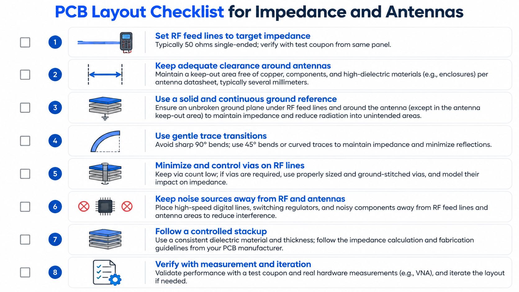
Layout is where the physics becomes copper. Each item below is one action and the reason it exists.
- Set RF feed lines to the target impedance, typically 50 ohms single-ended, and verify it with a test coupon cut from the same panel. A coupon from a different panel proves nothing about your board.
- Hold dielectric thickness and Dk constant across the stack-up. Small shifts move impedance, and a stack that changes mid-line creates a reflection you can't tune out later.
- Run a via fence on both sides of each RF line. The vias contain the field, cut leakage into neighbouring traces, and stop the line behaving like an unintentional antenna.
- Keep transitions short and straight. Right-angle bends and open stubs each add reflection, and at these wavelengths a stub a few millimetres long is a real discontinuity.
- Remove or back-drill via stubs that sit in the RF path. A stub acts as a notch filter at a frequency you didn't choose.
- Keep a continuous reference ground under the antenna and the feed lines. A split or slotted ground plane changes the impedance and radiates in directions you didn't design for.
<a id="antenna-thermal-and-finish"></a>
Antenna, thermal and finish
- Hold the antenna keep-out clear of copper pours, thick solder mask and, above all, enclosure metal. A steel screw 2 mm from a patch detunes it and reshapes the beam.
- Place decoupling capacitors close to the radar chip supply pins. The chip draws current in short bursts during a chirp, and a long supply loop turns that into phase noise.
- Give the chip a thermal path through the board to a heatsink or the enclosure. Radar ICs run warm, and Dk drifts with temperature, so heat is an RF problem as well as a reliability one.
- Specify surface finish and copper roughness with the fabricator. Both change loss at these frequencies, and neither is visible on a drawing unless you write it.
Two of these get skipped most often: the back-drill on a stub nobody modelled, and the antenna keep-out review with the mechanical team. Both surface as "the module underperforms" in the lab.
Detailed routing practice for mixed-signal boards carries over well, and this guide to high-speed PCB design covers the return-path habits that keep an RF section quiet.
Layout cannot fix a mechanical problem. Walk the enclosure drawing and the mounting position through the same review as the stack-up, because plastic thickness, paint and nearby metal change the antenna's behaviour more than any trace width decision will.
<a id="validate-the-stack-up-before-you-build-prototypes"></a>
Validate the Stack-Up Before You Build Prototypes
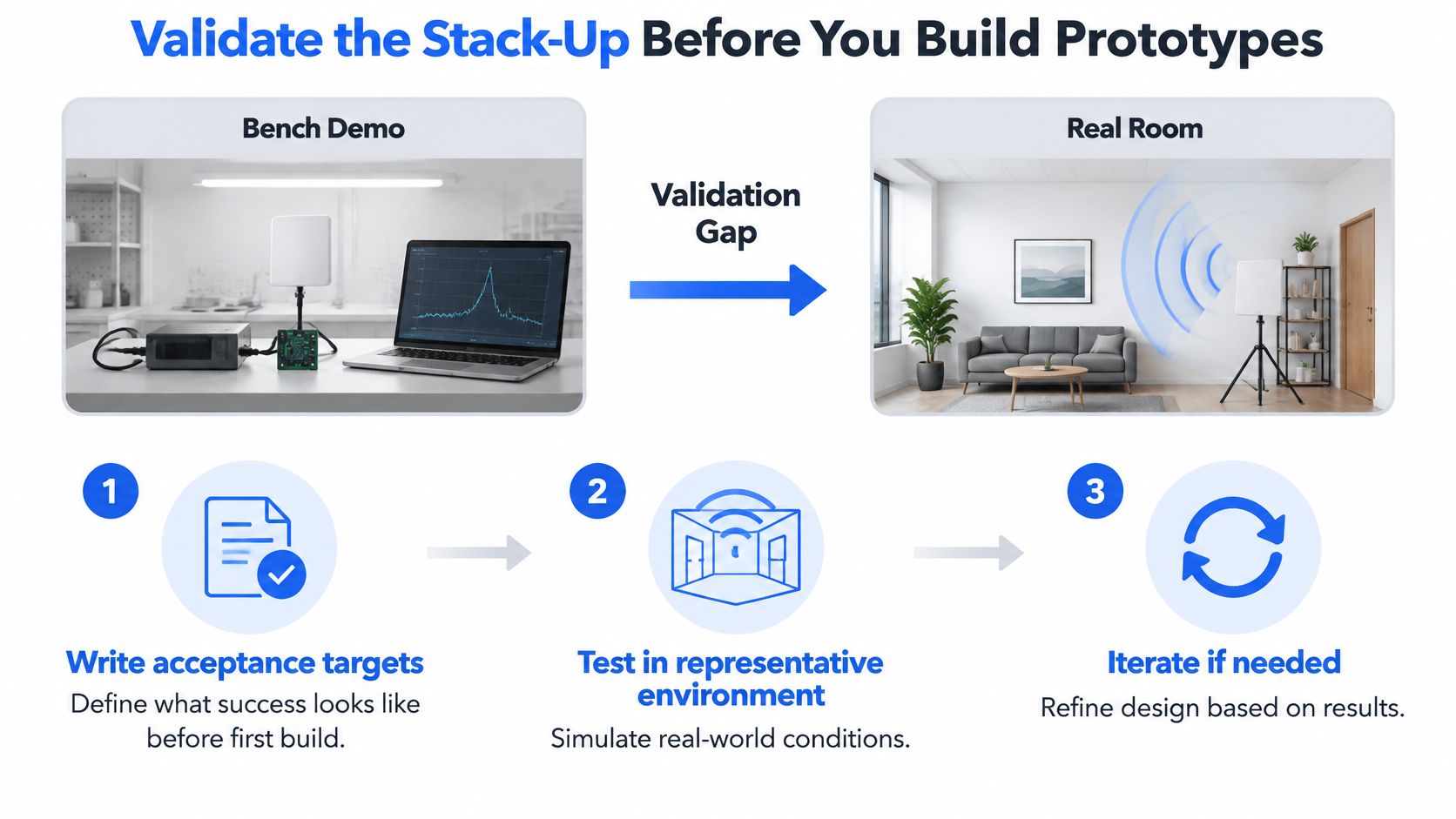
A clean bench demo proves the module works on a bench. It doesn't prove it works in a bedroom with a metal bed frame, a curtain and two people, so define what success means before the first build.
Set the sequence early and hold to it.
- Write acceptance targets for the intended use case. False alarm rate, missed detection rate and required coverage, in numbers, agreed by the product owner before layout freeze.
- Confirm regional spectrum and certification requirements for the chosen band before the prototype run, because a band that isn't permitted in a target market wastes an entire build cycle.
- Measure the test coupon on a vector network analyser to confirm impedance and loss while the layout is still changeable. After the panel is ordered, the measurement only tells you what went wrong.
- Test the complete assembly in its final enclosure and mounting position, using the same metal and plastic it will ship with. Bare boards flatter every design.
- Run ground-truth tests with several subjects, positions, distances, turns and movement patterns. Record confidence per detection so a weak result can trigger a fallback sensor or human review instead of a silent miss.
- Add production test points so every board can be checked after assembly, not just the first article.
- Run a small pilot batch and compare the results against the targets written in step one.
<a id="why-the-test-population-matters"></a>
Why the test population matters
A model tuned on tidy data fails in messy rooms. A 60 GHz vital-sign dataset published in Scientific Data states that age groups and health conditions are underrepresented, and that many studies collect subjects mainly at rest. Another dataset it discusses warns that radar point clouds may reflect clothing, moving limbs and surrounding objects rather than anatomical joints, and that testing often omits variable distances, turns, transfers, occlusion and larger cluttered rooms.
That's the practical trap. Higher resolution doesn't fix a narrow test set. Broader participants, realistic trajectories, calibrated ground truth and confidence estimates do more for a product than another gigahertz of bandwidth.
How much of the validation sequence can run at once? A good fabricator supports it directly. We build high-frequency PCBs on Rogers, PTFE and high-speed laminates with low Dk and Df, verified through SET2DIL, Delta-L and VNA measurement. We also inspect incoming material and run AOI, X-ray and flying probe testing on every board, so the sample you validate is the process you ship. Our layout group adds schematic capture, SI/PI simulation and DFM review in Altium, Cadence and Mentor.
Send the stack-up, layout files and enclosure drawing out for a DFM review before you commit to the first prototype run. It's cheaper to move an antenna 3 mm on a drawing than on a moulded housing.
Lianyuhong Technology Co.,Ltd fabricates high-frequency PCBs on Rogers, PTFE and high-speed laminates with controlled Dk and Df, verified by VNA, SET2DIL and Delta-L measurement, and inspects incoming material before AOI, X-ray and flying probe testing on every board. Our layout team covers schematic capture, SI/PI simulation and DFM review in Altium, Cadence and Mentor, so the impedance target, the antenna keep-out and the enclosure drawing get checked together rather than in sequence. Bring us your stack-up and mechanical drawing for one joint review and see what changes before the first panel is cut, starting at Lianyuhong Technology Co.,Ltd.